Authors:
(1) Yuxin Meng;
(2) Feng Gao;
(3) Eric Rigall;
(4) Ran Dong;
(5) Junyu Dong;
(6) Qian Du.
Table of Links
- Abstract and Intro
- Background
- Proposed Method
- Experimental Results and Analysis
- Conclusions and Future Work
- References
IV. EXPERIMENTAL RESULTS AND ANALYSIS
A. Study Area and Experiment Settings
The South China Sea is located in the Western Pacific Ocean, in southern mainland China. Its area is about 3.5 million square kilometers with an average depth of 1, 212 meters. In this paper, the selected study area is (3.99°N∼24.78°N, 98.4°E∼124.4°E).
We use the high-resolution satellite remote sensing data from GHRSST (Group for High Resolution Sea Surface Temperature) [55] as the observed data. GHRSST provides a variety of sea surface temperature data, including satellite swath coordinates, gridded data, and gap-free gridded products. Herein, we have employed gap-free gridded products, which are generated by combining complementary satellite and in situ observations within an Optimal Interpolation framework. The HYCOM [56] is selected as the numerical model. Their spatial resolutions are 1/20°×1/20° and 1/12°×1/12°, respectively. The temporal resolution is one day. The data from May 2007 to December 2013 are used for training, while the remaining data from January 2014 to December 2014 are used for testing. It should be noted that we use cloudless data provided by GHRSST. The data were captured by microwave instruments which can penetrate through clouds. Hence, the data have full coverage of the study area. In addition, the accurate time of every pixel in GHRSST SST product is the same.
The Z-score standardization was utilized for preprocessing as:

where x denotes the GHRSST and HYCOM model SST, z denotes the normalized data, µ and σ denote the mean value and standard deviation respectively. We converted the data into 256 × 256 square-shaped heat maps.
More specifically, the GHRSST data and 512-dimensional random vector are utilized in the first step of prior network training. The size of the input GHRSST data is N × H × W, where N represents the batch size, H indicates the height of the input data, and W denotes the width of the input data. For the second stage of prior network, we only employ GHRSST data for encoder training. The sizes of inputs and outputs for both stages are N × H × W. Similarly, in the third step of prior network training, the HYCOM SST data is fed into the pretrained model. Here, the sizes of both the inputs and the outputs are N × H × W. In our implementations, we set N to 2430, while H and W are both set to 256.
We conducted extensive experiments on an NVIDIA GeForce 2080Ti with 8 GPUs. The prior network uses the same network structure and configuration as mentioned in [53] to acquire the physical knowledge from the historical observed data. Then the obtained physical knowledge is transferred to the numerical model data for the sake of restoring and improving the incorrect components in the numerical model. The configuration for the ConvLSTM model used in this paper is the same as the ConvLSTM model in Shi’s work [20]. The GHRSST SST dataset is utilized as the benchmark for comparison and assessment in this paper.
B. Influences of the Past Day Number for SST Prediction
As mentioned in Section III. C, t denotes the number of past days used for prediction. It is a critical parameter that may affect the SST prediction performance. In this paper, we attempt to predict the next one-day, three-day and sevenday’s SST. We implemented extensive experiments to find the

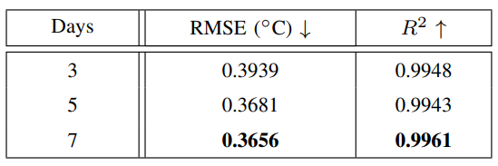

proper number of past days for the future SST prediction. The Root Mean Square Error (RMSE) and the coefficient of determination (R2) are applied as the evaluation criteria. Lower RMSE and higher R2 values indicate more accurate results.
Table I lists the prediction results for the next day by using the past one day, three days and five days’ data, separately. It can be observed that the proposed model performs best when using the past five days’ data, where the RMSE and the R2 results are 0.3618 and 0.9967 respectively. They are slightly better than the other schemes. Compared to the other two schemes, the RMSE and R2 values improve by 0.0086, 0.001 and 0.0028, 0.0006. Hence, the past five days’ data are adopted for the next one-day SST prediction.
We analyze the influences of t for the next three-day SST prediction in Table II. It can be seen that the longer historical data was used, the better prediction performance was achieved. The RMSE value using the past seven days’ data achieves the best performance. It is improved by 0.0025 compared to that using the past five days’ data. Meanwhile, the R2 performs the best using the past seven days’ data compared to the other two schemes. Therefore, the past seven days’ data were used for the next three-day SST prediction.
The experimental results of the next seven-day SST prediction is illustrated in Table III. As can be seen that the prediction results using the past ten days’ data achieves the best performance. Therefore, we exploit the past ten days’ data for the next seven-day SST prediction.
C. Ablation Study
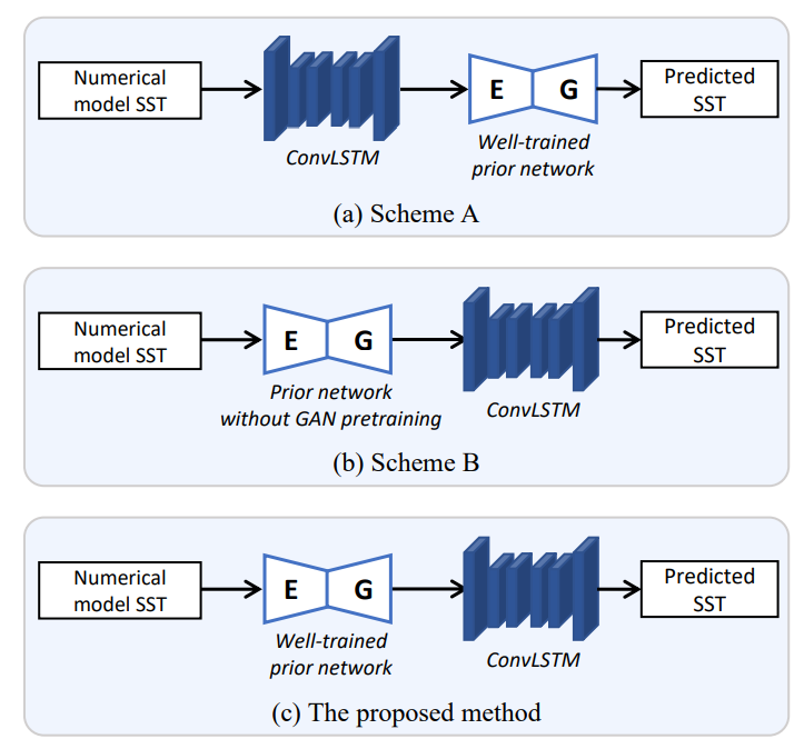
To verify the effectiveness of the prior network and GAN training, we conduct ablation experiments. As illustrated in Fig. 3, two variants are designed for comparison as follows:
• Scheme A. The sequence of prior network and ConvLSTM is replaced. The numerical model SST data are first fed into the ConvLSTM, and then the output are fed into the well-trained prior network.
• Scheme B. The prior network has not been well-trained. Specifically, GAN model training (the first step in Fig. 2) in prior network training has been omitted.
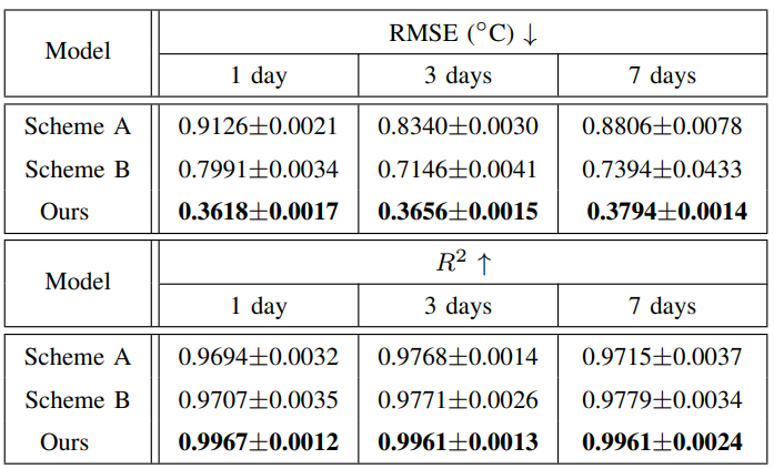
The experimental results are shown in Table IV. As can been seen that our method achieves the best RMSE and R2 values. Specifically, the proposed method outperforms Scheme A, which demonstrates that the correct sequence of prior network and ConvLSTM can boost the SST prediction performance. It is evident that the prior network effectively restores the incorrect components of the numerical model data, and the restored data perform better in SST prediction. Futhermore, the proposed method has superior performance over Scheme B, which demonstrates that the GAN modeling is an essential step. GAN modeling can learn the data distribution of the observed SST, and helps the prior network capture better physical information from the observed SST. To sum up, in the proposed method, we use adversarial learning for prior network pretraining, which can effectively transfer physical knowledge from the observed SST data to the prior network. It can guide fast training convergence, and improve the SST prediction performance.
D. Experimental Results and Discussion
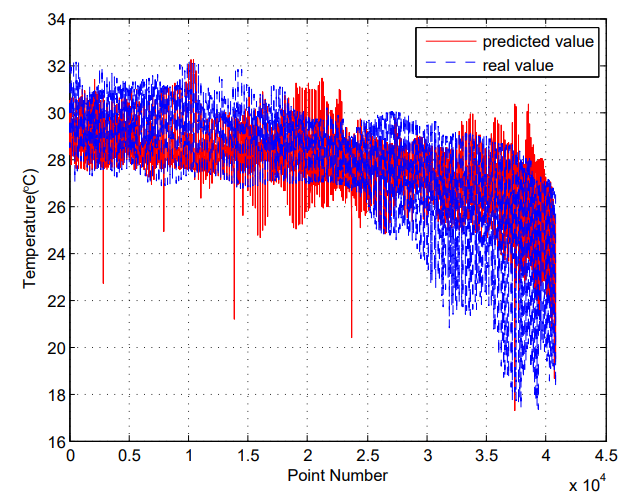
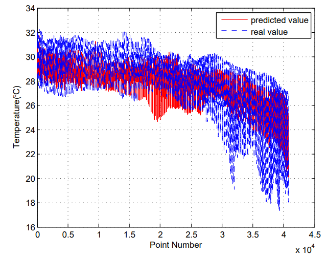
Fig. 4 compares the predicted next one-day SST with the observed ground truth data. We can see that the predicted results of our method match well with the observed data. Similarly, the observed data and the corresponding predicted SST for the next three days and seven days are displayed in Fig. 5 and Fig. 6, respectively. The visualized results indicate that the proposed method can generate robust and reliable results for SST forecasting.
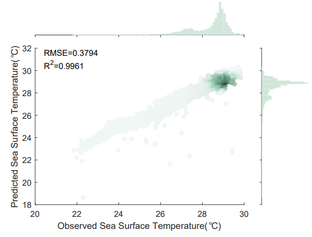
A scatter plot on the SST prediction for the next one day is illustrated in Fig. 7. It can be observed that the data points are
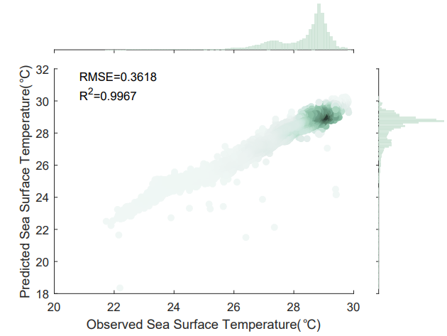
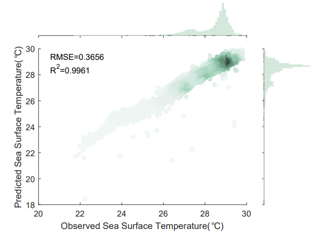
roughly evenly distributed near the red line. Fig. 8 and Fig. 9 are scatter plots of the prediction results for the next three days and the next seven days, respectively. The scatter plots demonstrate the effectiveness of the proposed method for SST prediction.
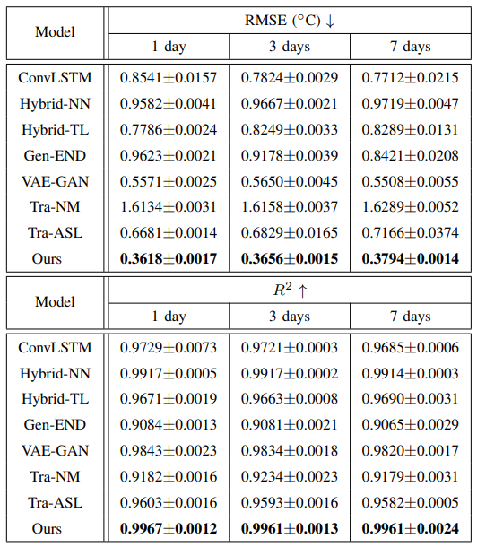
In order to verify the effectiveness of the proposed method, we compare the proposed method with seven closely related methods: ConvLSTM [20], Hybrid-NN [14], Hybrid-TL [15], Gen-END [57], VAE-GAN [58], Tra-NM, and Tra-ASL. The study area is (3.99°N∼24.78°N, 98.4°E∼ 124.4°E) for these methods. All of these methods used the training data from the past 5 days for the next 1-day prediction, the data from the past 7 days for the next 3-day prediction, and the data from the past 10 days for the next 7-day prediction.
ConvLSTM is discussed in Section III. C, and it is an effective spatial-temporal model for SST prediction. HybridNN utilizes the discrepancy between the observed data and the numerical model data to guide the training of deep neural networks. Hybrid-TL combines the advantages of numerical models and neural networks through transfer learning. GenEND is a generative encoder that can be used for SST prediction. VAE-GAN integrates variational autoencoder and
GAN, and it can capture high-level semantic features for SST prediction. HYCOM SST data are used to train the ConvLSTM model for the next 1-day, 3-day, and 7-day prediction (termed as Tra-NM). Tra-ASL is a traditional assimilation method and it exploits the correlations among multiple types of data (observed data and numerical model data).
The GHRSST data is first utilized to train a ConvLSTM model, which serves as the baseline. It is a widely used data-driven approach for SST prediction. Hybrid-NN, HybridTL, Gen-END, and VAE-GAN employ the GHRSST and HYCOM data for training. The HYCOM assimilation data [56]

are used here, with a spatial resolution of 1/12°×1/12°. Our method improves and rectifies the incorrect components in the numerical model data by introducing physical knowledge from the historical observed data. The corrected numerical model data is referred to as the physics-enhanced data. To compare with the physics-enhanced data, HYCOM assimilation data (Tra-ASL) and HYCOM data (Tra-NM) are similarly used to train the ConvLSTM model.
The training times of ConvLSTM, Hybrid-NN, Tra-NM, and Tra-ASL for the next 1-day, 3-day, and 7-day predictions are 1.8, 4.4, and 8.2 hours, respectively. The Hybrid-TL method trained the ConvLSTM model twice, and the training duration is 3.6, 8.8, and 16.4 hours for the three tasks, respectively. The VAE-GAN requires 181.6, 184.2, and 188.4 hours for training, while the Gen-END method requires almost the same amount of time, with 196.8, 199.3, and 203.2 hours for three SST prediction tasks, respectively.
The results for the next 1-day, 3-day, and 7-day SST prediction are presented in Table V. It is evident that the TraNM method yields unsatisfactory results compared to the other methods. This is likely due to the incorrect components in the HYCOM data, which adversely affect the SST prediction performance. The Hybrid-NN method also performs poorly, as its average RMSE values are the second lowest among the models. The Hybrid-TL model performs better than the ConvLSTM for the next 1-day SST prediction, but not for the other two tasks. Our method achieves the best RMSE values and highest R2 values. Compared to the ConvLSTM model, the average RMSE values of our method are effectively improved. It demonstrates that introducing physical knowledge
from the observed data can restore the incorrect components in the numerical model data, thus improving the SST prediction accuracy.
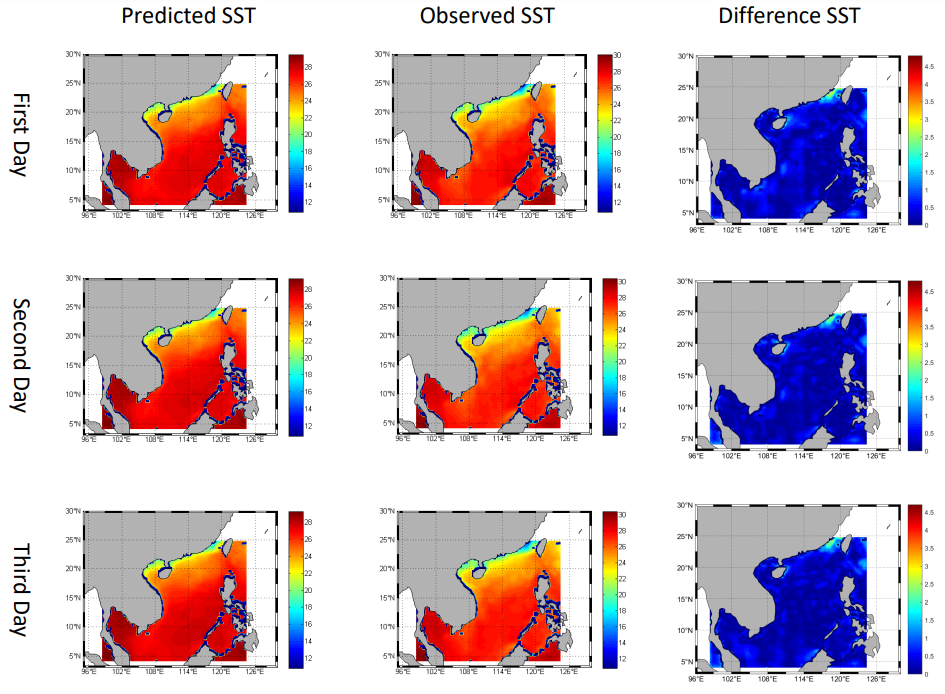
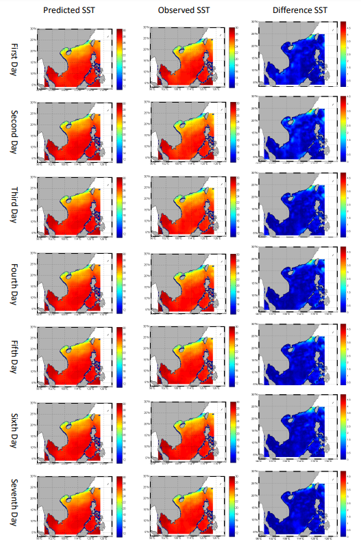
Fig. 10 presents the visualized results for the next one-day SST prediction, the observed SST data, and their differences, respectively. It can be seen that the predicted results are highly similar to the observed SST data across the entire region of the South China Sea. Fig. 11 displays the visualized results for the next three-day SST prediction. It is observed that there are some significant difference values in the Gulf of Tonkin and in other marginal areas of the South China Sea. Fig. 12 illustrates the visualized results for the next seven-day SST prediction. It is found that the major difference values mainly concentrate on the Gulf of Tonkin for the next seven-day prediction, and they are larger than the results for the two other tasks.
E. Limitation and Discussion
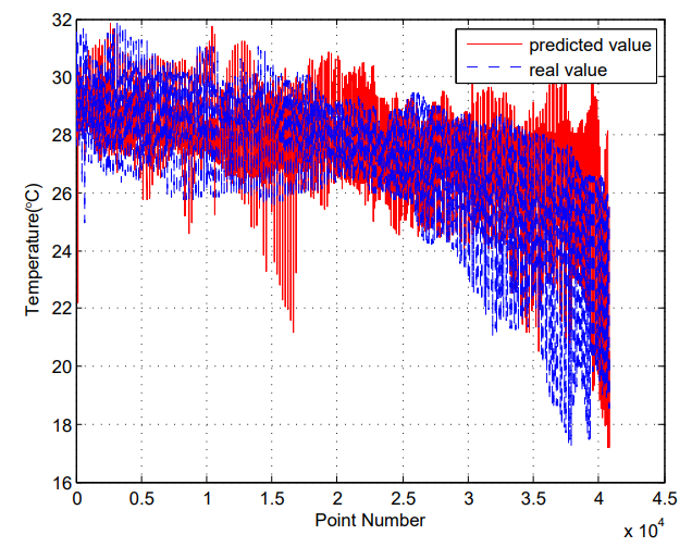
From Fig. 7 to Fig. 9, it can be observed that there are some inaccuracies in the mid-range SST, which are visualized in Fig. 13. Bright pixels indicate large SST prediction errors, whereas dark pixels denote accurate SST predictions. As can be seen, these points are mainly located on the northwestern part of Taiwan Strait, where the predicted sea surface temperature is lower than the observed data. The prediction error is mainly caused by the ConvLSTM model and the land mask. In our implementations, the land mask is applied to the study area. The ConvLSTM exploits the spatial and temporal features of the whole study area. The features of the northwestern part of Taiwan Strait are affected by the land mask to some extent, and therefore result in prediction errors. If higher resolution training data could be obtained, the accuracy of predictions in this region would be further improved.
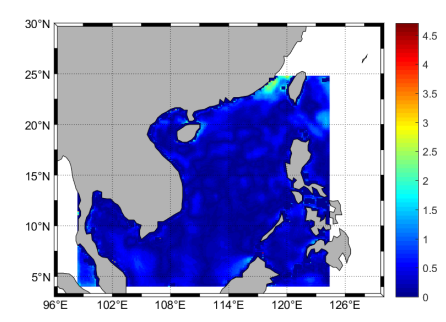
In Fig. 11 and 12, it can be seen that there is no significant increase in errors with the lead day. This may be due to the fact that our method uses a sufficient amount of training data, and the deep neural networks are able to effectively capture the temporal features. Furthermore, the persistence of SST is also an important factor.
This paper is available on arxiv under CC 4.0 license.

